Editors

Most of the editors can be accessed from the menus, or by clicking the associated icon on the design toolbar.

Delivery Point editor

Defining a delivery point is the first step in building a gathering system. When selecting the location of the delivery point, it is important to consider the objectives of the modeling work. Good locations for delivery points are custody transfer points, discharge or suction of compressors, or any other point where flowing pressures are expected to remain constant for the study period.
Click the standard gas processing plant icon for delivery points in the gathering system, regardless of whether the delivery point is a plant, compressor, contract, sales meter, etc.

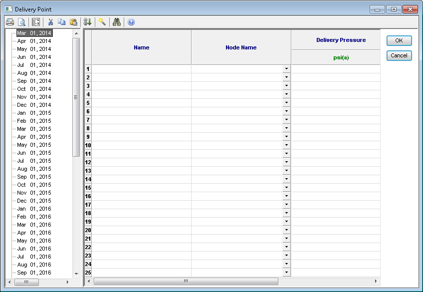
If you need to build a more complicated system containing two or more delivery points, you can specify each separate delivery point within the system in the Delivery Point editor. For a single file, you must define at least one delivery point, up to a maximum of 25 delivery points. For both GIS and Cartesian modes, you can create, modify, and delete delivery points in this editor.

Delivery point name

The delivery point name is the name given to the primary or starting node in a gathering system. By default, delivery point names are “Delivery Point 1”, Delivery Point 2”, etc. We recommend that you change your delivery point names to reflect specific locations in your system.

Note:

You can adjust the node / facility naming convention in the facility name generator configuration.

Plant delivery pressure

The delivery pressure is the pressure assigned to the outlet of the delivery point. Revise the default delivery point pressure of 900 psia (6205 kPaA) to reflect the delivery pressure of the system, or portion of the system being modeled. Note that the minimum allowable value for delivery pressure is 5 psia (35 kPaA).

This pressure can be scheduled through time to reflect seasonal delivery pressure variations or scheduled changes to compression suction pressure.

Note:

Your model's pressure-loss calculations require appropriate delivery point pressures.

GIS Positions editor

Use this editor to define location information for nodes in GIS mode. You can also attach nodes to facilities (for example, a well, compressor, separator, etc), but only one facility can be attached to a node.

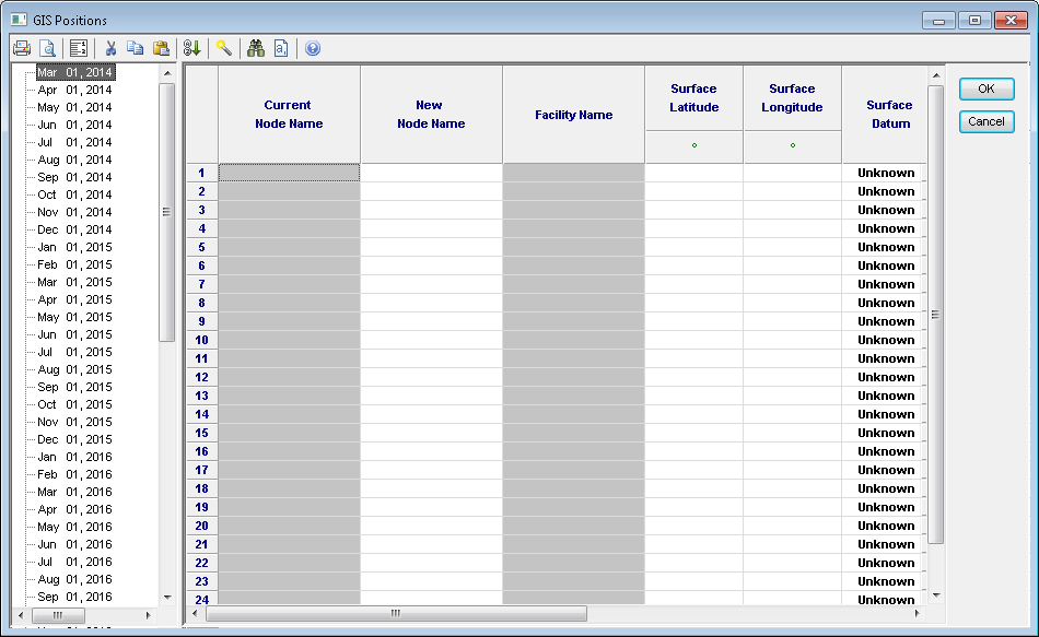
In this editor, you can define the name of the node, along with the type of facility, if any, that is attached to that node. You can also define the coordinate systems (latitude / longitude, DLS, NTS, and UTM). If you would like to display other coordinate system data, right-click the columns with in the GIS Positions editor and select Show Extra Location Columns.

Note:

Nodes that are attached to wells have a sandface location associated with them, and the sandface location can be different from the wellhead location.

These rules apply to this editor:

• In GIS mode, you can define a node in the GIS Position editor. Or, you can use the Gathering System editor, but the node is not assigned coordinates. To remove or attach facilities to nodes, use the Facility editor.
• In GIS mode, you can only change the node name with the GIS Position editor. Changing the name of the node applies changes to attached facilities and gathering system linkages.
• If a change is made to any of the location coordinates for a node, other location coordinates for that node will be updated to reflect that change. (Changes override the existing location, regardless of which coordinate system the change is made for.)
• If changes are made to more then one coordinate system and those changes are inconsistent, the following hierarchy determines which coordinate system takes precedence :
• Latitude/Longitude
• UTM
• DLS
• NTS

• You can enter measured pressure values, so that you can compare forecasted values to determine if there are discrepancies between the actual pressure and the simulated pressure.

• Elevation values are entered in absolute values to convert the elevation differences in the Gathering System editor.

Node editor

Use this editor to view and change node names and facilities attached to the node in Cartesian mode.

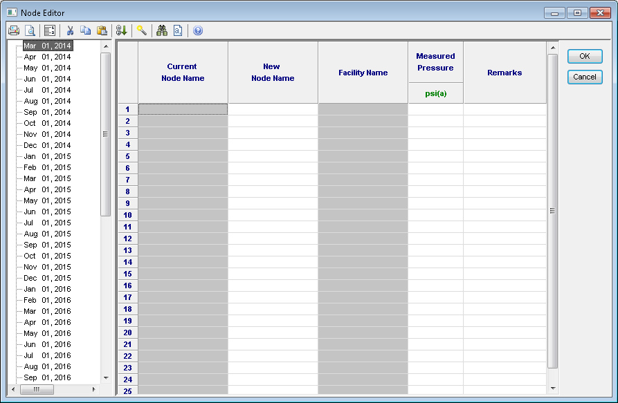
These rules apply to this editor:

• You can define nodes in the Node editor, or the Gathering System editor (provided that the node is linked to a node existing in the Cartesian space). To removing or attach facilities to nodes, use the Facility editor.
• In Cartesian mode, you can only change the node name in the Node editor. Changing the name of the node applies changes to attached facilities and gathering system linkages.
• You can enter measured pressure values, so that you can compare forecasted values to determine if there are discrepancies between the actual pressure and the simulated pressure.

Gathering System editor

This editor is used to create the overall superstructure of the gathering system. Once the structure has been defined, facilities (wells, compressors, etc) can be assigned to specific locations within the system.

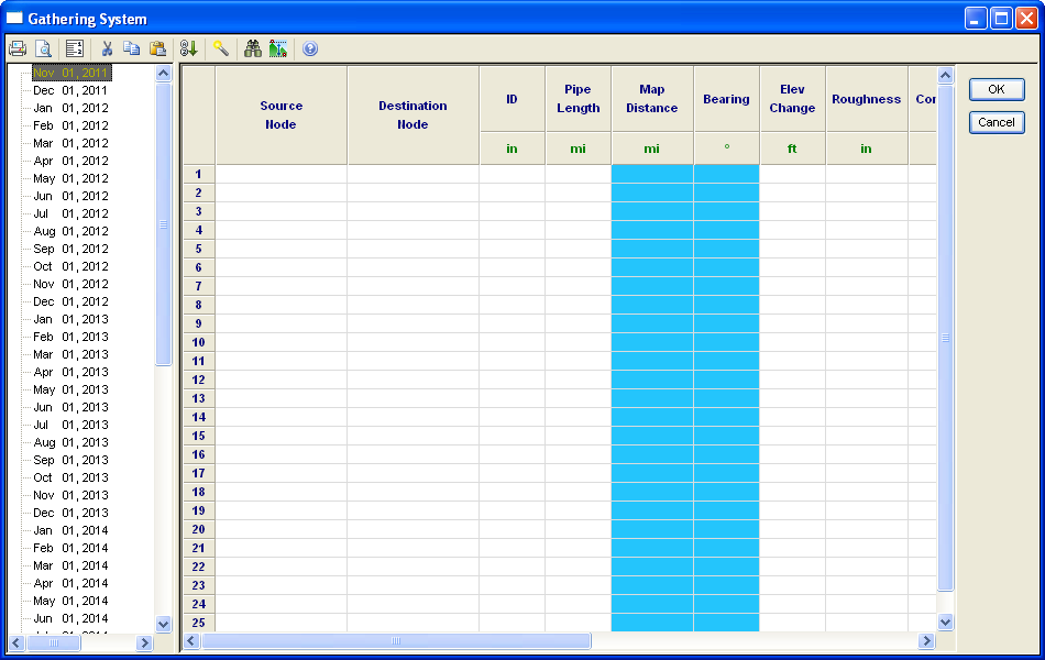
When a row is highlighted blue, it has become disabled and becomes a thick black line on the GIS map. This happens when a loop has been formed but a valid Loop Link has not been designated. Designate a valid Loop Link or remove an invalid link and turn off the Disable Link flag.

(A) Required editor inputs

Source node

Starting point of a pipeline segment

Destination node

Endpoint of a pipeline segment

Pipeline length

A non-zero length is required for any pipeline segment. For more information, see pipe length vs. map distance.

Map distance (not accessible by the user)

The actual distance of the pipeline segment on the GIS map.

Bearing (accessible in Cartesian mode only)

Reflects the angle between the source and destination node that define the linkage. For more information, see bearing.

(B) Optional parameters

Pipeline ID

This is the inside diameter of a pipeline. If no pipeline ID is specified, Piper does not calculate a pressure drop along the length of the pipeline segment.

Elevation change

You may want to include topographical elevation changes in the case of hilly terrain, or when dealing with multiphase flow. The sign convention is shown below:

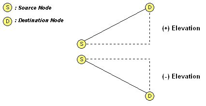
So, if the source node is lower than the destination node, then the elevation is positive(+). If the source node is higher than the destination node, the elevation is negative(-). The flow direction should not be considered when entering the elevation changes.

If there are absolute elevations entered in the GIS Positions editor, the elevation change can be automatically calculated by clicking the icon in the Gathering System editor.

Pipe length vs. map distance

Because of the change to geodetic locations in Piper, the length column in the Gathering System editor has been replaced by two lengths: pipe length and map distance.

• Pipe Length: This is the length that is used to calculate the pressure loss in a pipeline segment. The pipe length can reflect the undulations and turns in the pipeline that may cause the true length of the fluid flow to differ from the geodetic distance between two points.
• Map Distance: This reflects the distance between the two nodes that define the link as is calculated from the latitude and longitude location of each node. You cannot change the map distance. If the latitude and longitude of a node is changed either on the map or through the GIS Position editor, the map distance will automatically update to reflect that change.

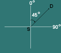
Bearing

Angles are assigned between two points using a polar coordinate system. The bearing reflects the angle between the source and destination nodes that define the linkage. Like map distance, the bearing is determined based on the geodetic location that defines the linkage, and cannot be changed in the Gathering System editor when in GIS mode. If the location of either of the nodes is changed, the bearing will automatically update to reflect this change.

Note:

Bearing is defined based on 0 degree as true north.

Loops

Incorporating line loops into a model can cause confusion with new users. Below is a brief description of looping with suggestions on how to incorporate loops into a model. If you need clarification, please contact us.

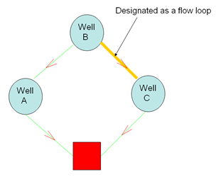
A pipeline loop provides an alternate route for gas to flow. Loops are installed in order to increase pipeline capacity. Two types of looping structures can be made in Piper: line loops and flow loops. In order to designate a line / flow loop, the line must be specified in the Gathering System editor using the columns below:

Looped: indicates if the pipeline segment is a loop
Unique ID: distinguish between various loop lines, if multiple loop lines are present.

Line Loop (twinning a line)

Flow Loop (alternate direction for gas to flow)

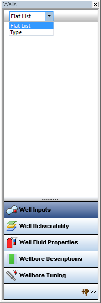
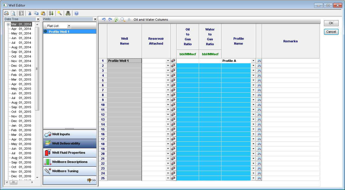
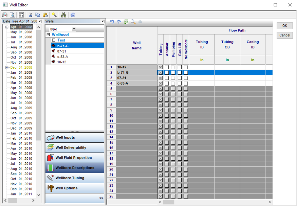
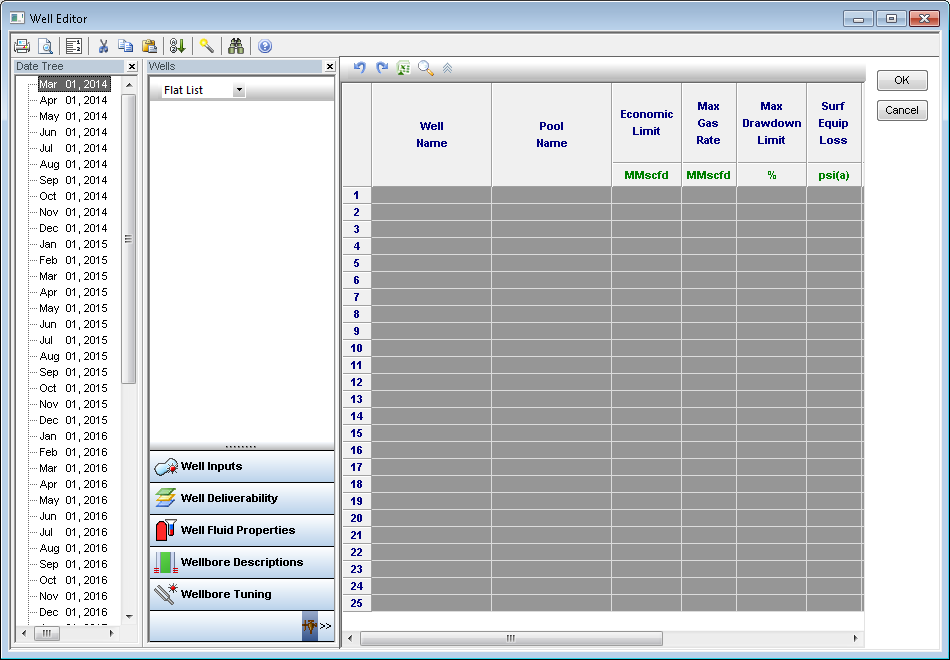
Well editor

This editor is used to specify how well production is modeled over time, and consists of three sections: Date Tree, Well Manager Model Manager, and the Well Viewer.

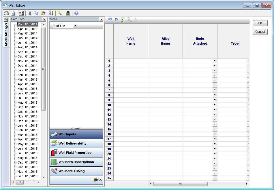
Date Tree: in this section, you can navigate through the configuration dates.

Wells Manager: in this section, you can view and navigate through the list of wells. At the bottom of this section, you can configure different parts of a well.

• Well Inputs
• Well Deliverability
• Well Fluid Properties
• Wellbore Descriptions
• Wellbore Tuning
• Well Options

The Well Manager sorts the wells in the model using two options: Type and Flat List.

Well Viewer: in this section, you can control the data displayed in the Well Viewer editor.

Well inputs

If you use a well name that corresponds with a node name for the pipeline network, a well is created at that node location.

Well Name: the name of the well

Alias Name: an alternative name for wells, so that during importing Piper can update data.

Node Attached: wells can be assigned to existing nodes by clicking the drop-down arrow to the right of each field in the Node Attached column. A list of existing nodes is displayed. To assign a well to a node location, click the desired node name.

Or, a new node name can be defined in the Node Attached column. However, if you create a new node this way, you need to specify a location in the GIS Position editor.

If the node name is left blank, the deliverability data defined for that well remains in the Well editor, but the well is not located on-screen and exists as an unused facility.

Type: the performance of the well is determined by the type of well selected in the Type column. Deliverability options are assigned by clicking the drop-down arrow and selecting from the list. For more information, see Deliverability Options.

On-stream Date: you can create a well on one configuration date and activate it on a later date. When a well is on-stream it is displayed on the map as a colored well (), and a well that is off-stream is displayed as a gray well () on the GIS map. During forecasting, an off-stream well will not produce until it reaches it's on-stream date. If an on-stream date starts before the forecasting period, then the well is producing.

Note:

Although a well can have an on-stream date before the forecast period begins, Piper does not calculate the deliverability of the well for the period before the forecast period. The well starts producing on the first forecast date, if the on-stream date is set before the forecast date.

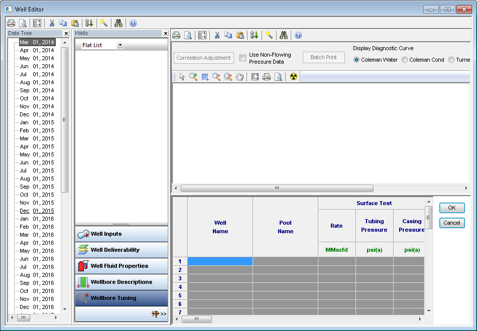
Well deliverability

Well deliverability is used to specify how well production is modeled over time. Using a well name that matches a node name within the pipeline network results in a well at that node location. In Piper, deliverability is assigned on a well-by-well basis. The Type column in the Well Inputs editor is used to assign a type of deliverability for a well. For any selected delivery type, white fields indicate that data input is required, and fields that do not require input are highlighted in blue.

Reservoir Attached: some wells require an attached reservoir. You can assign a reservoir name to either an individual well or a group of wells by clicking the drop-down arrow to the right of each field in the Reservoir Attached column. To assign a reservoir to a well, click the appropriate reservoir name.

Deliverability options

These are the main categories for defining the deliverability of a well:

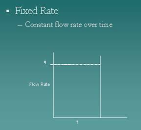
1. Fixed Rate - defines the deliverability of a well as a constant gas rate over time. The gas rate remains fixed despite changes in reservoir or pipeline pressures. Note that a reservoir does not need to be designated to a fixed rate well. However, if a reservoir is assigned to a fixed rate well, the well produces at the specified gas rate until the reservoir volume is depleted.

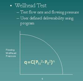
2. Wellhead Test - defines the deliverability of a well at the wellhead. A flowing wellhead gas rate, corresponding flowing pressure, and wellhead ’n’ value are required for input. In addition, a reservoir must be assigned to the well.

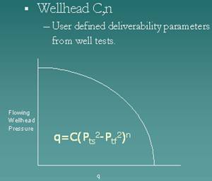
3. Wellhead C, n - defines the deliverability of a well at the wellhead. A wellhead ’C’ and wellhead ’n’ value are required for input. These parameters are available from AOF / backpressure / deliverability tests. In addition, a reservoir must be assigned to the well.

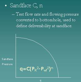
4. Sandface C, n - defines the deliverability of a well at the sandface. A sandface ’C’ and ’n’ value are required for input. These parameters can either be entered (from deliverability test information), or they can be calculated in the Wellbore Tuning editor.

5. Transient - defines the deliverability of a well by selecting one of the various simplified analytical reservoir models. The required inputs for transient wells are completed in the analytical well editors. See Analytical Models for more information.

6. Profile - defines the well deliverability through time based on user-supplied production decline profiles. A well modeled using this option produces according to the user-defined trend and is not affected by changes in well back pressure. You must enter the profile name in the deliverability editor, and this name must first be defined in the Profile editor. For more information, see Profile Editor.

For a more detailed description of modeling and options, see wellbore tuning for sandface deliverability wells.

Profile editor

To open the Profile editor, click the Profile icon () in the Profile column. (You may have to scroll horizontally to see this column in the table.) In this editor, you can create or import a production profile, which can be assigned to an individual well.

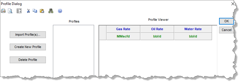
To create a new production profile, click the Create New Profile button. The following inputs are required:

• Profile name
• Gas rates and Liquid rates — can be entered in the Profile Viewer, or content can be brought in from an Excel file.

A production profile can be imported from an existing .csv, .txt, or .xlsx file by clicking the Import Profile(s) button and specifying the file to import. After a profile has been made, it can be assigned to the appropriate well(s) in the Well Deliverability Editor. We recommend selecting the Profile option in the Well Deliverability editor, and assigning a profile name from the drop-down menu.

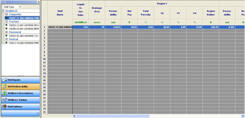
Analytical models

Analytical models are used to predict reservoir deliverability. To use this editor, assign a well a transient deliverability in the Well Inputs editor. The required inputs are shown in white.
There are five types of analytical models, and the Well Editor has a different table / grid for each model.

1. Legacy Transient: The legacy transient models consists of four different model types. These model types are simplified approximations of the rate transient analysis (RTA) analytical models of the same type. Specifically, the legacy models do not consider the effect of superposition of pressure. Therefore, these models could be expected to under predict the rate changes caused by changes in pressure.

2. Vertical: represents a vertical well in a rectangular, homogenous reservoir.

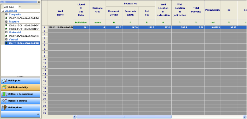
3. Fracture: represents a model of a single fracture off a vertical wellbore in a rectangular reservoir.

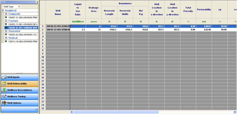
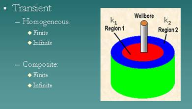
4. Composite: represents a vertical well in a circular reservoir with an inner circle with one set of properties and an outer circle with another set of properties.

5. Horizontal: represents a single horizontal leg off of a vertical wellbore in a rectangular reservoir.

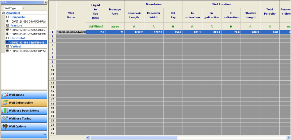
For each option, you must enter an on-stream date and reservoir parameters.

For more information on the parameters used to define each well type, see the Analytical Model.

Well fluid properties

The Well Fluid Properties editor's table / grid is accessible from the Well editor.

The contents of the well fluid properties depend on whether you have selected Black Oil, Peng-Robinson / Wilson, or for no-phase volume calculations to be performed.

For more information on how to use well fluid properties, see Defining Compositions.

Wellbore descriptions

With this editor, you can:

• Specify the type of completion
• Enter wellbore dimensions
• Model wellbore loading and pumping
• Select a correlation for calculating wellbore pressure losses

For any option selected in this editor, white fields indicate required inputs, and blue fields indicate parameters that are not required. To model a wellbore in Piper, you have five major options available:

1. Tubing

This option requires you to enter the tubing inner diameter (ID) and outer diameter (OD), along with the casing ID. You must also enter end of tubing (EOT) and the mid-point of perforations (mpp). With these values entered, wellbore calculations take place along the tubing until EOT is reached, and then either up to mpp in the annulus, or down to mpp in the casing. The wellhead pressure is determined from the surface gathering system. You can also specify the wellbore pressure loss correlation, if you want to change it from the default value.

Note:   With Piper, it is assumed that tubing exists in your well. If your well does not have tubing (i.e., casing-only flow path), we recommend that you enter your actual casing inner diameter as "Tubing ID", and then enter larger dummy values for "Tubing OD" and "Casing ID".

2. Annular

This option requires you to enter a tubing ID and outer diameter OD, along with the casing ID. You must also enter EOT and mpp. With these values entered, wellbore calculations take place along the annular flow path until mpp is reached. If mpp is deeper than EOT, then wellbore calculations take place along the annulus until EOT, and then use the casing diameter to mpp. The wellhead pressure is determined from the surface gathering system. You can also specify the wellbore pressure loss correlation, if you want to change it from the default value.

3. Pumping

Piper uses the pumping flow path in a similar way to Harmony and Harmony Enterprise. In general, gas is assumed to flow up the annulus, while liquid is pumped up the tubing. Since there is no ability in Piper to calculate the pressure drop across the pump (in the tubing), all wellbore pressure loss calculations are performed in the annulus / casing. This is done in two stages:

• Stage 1: calculates the pressure drop from the wellhead to the liquid level using a single-phase gas method
• Stage 2: calculates the pressure drop from the liquid level to mpp using a gradient calculation

Note:   The liquid level is entered using the Fluid Column Height.

- Fluid Column Height — this is the constant height of the fluid column above the EOT, and it is needed to maintain proper pump operation. You can edit the default value of 250 ft.

- Gasified Liquid Column Gradient — this parameter is used to calculate the back pressure imposed on the formation by the column of fluid you previously specified. You can edit the default value of 0.265 psi / ft.

The pumping flow path can be enabled either at the beginning of a well's life, or after liquid loading begins. For the latter option, you want to choose a Liquid Lift Correlation, and then Submersible pump as the method used after the well loads.
By default, Piper assumes that the wellhead pressure obtained from the surface gathering system is the casing / annulus wellhead pressure for the pumping flow path. If the surface gathering system is connected to the tubing output, you need to manually enter the wellhead pressure at the casing / annulus. If so, enable Use Casing Pressure and then enter the pressure you want for wellbore calculations.

4. Gas Lift

Piper uses the gas lift flow path in a similar way to Harmony and Harmony Enterprise. In general, this flow path is related to the tubing flow path described earlier, but with additional gas in the tubing part of the wellbore. The math can be described in two stages:

• Stage 1: calculates the pressure drop from the wellhead to EOT using both reservoir gas and injected gas-lift gas, along with any liquids produced by the reservoir.
• Stage 2: calculates the pressure drop from the EOT to mpp using exclusively the reservoir fluids.

The injected gas lift rate can be set in one of two ways:

• Using a Gas Lift Profile
• - Requires you to enable a Use Gas Lift Profile (this profile must be created and selected in the drop-down list). Creating a gas lift profile is similar to creating a production profile for a Profile Well.
• - When you enable this feature, Piper adds the gas lift profile rate for each time step to the produced rate for that same time step.
• Using a Gas Lift Gas Rate Factor
• - Requires you to enter a Gas Lift Gas Rate Factor, and select a liquid lift correlation from the drop-down list in the Liquid Lift Correlation column.
• - When you enable this feature, Piper calculates the minimum rate necessary to lift liquids, and multiplies that rate by the entered Gas Lift Gas Rate Factor.
• - The calculated gas lift rate is then added to the produced gas rate.

Note:   The gas gravity of the injected gas-lift gas uses the default value of 0.65. You can change this by clicking the Gas Lift Compositions icon.

5. No Wellbore

Piper has an option to ignore the frictional and liquid pressure losses. With this option, Piper only considers a static gas column within the wellbore. This option is intended to mirror the results for wells imported from previous versions of Piper where the wellbore was not specified.

If you choose to use No Wellbore, the only inputs this option requires are the mpp and the single-phase correlation. Sandface pressure is calculated assuming static gas from the surface to mpp.

For a more detailed description of modeling and options, see Wellbore Tuning Reference Materials.

Wellbore tuning

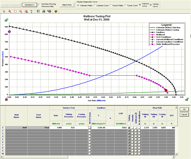
With this editor, you can create and modify the parameters for sandface wells.

To create a Sandface Deliverability well, enter either input a Sandface 'C' and 'n' value directly, or enter a Surface Test Pressure, Test Rate, and Liquid to Gas Ratio (LGR), from which Sandface 'C' can be calculated. If you do not specify an n value, a default value of n = 1 is applied.

This editor has following additional functionality:

• Enter and adjust Wellbore Flow Path dimensions. Or, Wellbore Flow Path dimensions entered in the Wellbore Description editor will be automatically retrieved.
• Use the Turner or Coleman liquid lift correlations to determine the ability of the well to lift liquids to surface and simulate metastable flow rates after the onset of loading.
• Adjust the Gasified Liquid Gradients in the Casing and Tubing / Annulus to tune the well to the desired post liquid loading performance.
• Automatically switch a well that becomes unable to lift liquids to artificial lift.

Methods of using the wellbore tuning editor to calculate sandface C

If the sandface deliverability of a well is known, you can enter it in the Sandface C field. If the sandface deliverability is not known, the deliverability can be calculated in different ways:

• If the well is able to lift liquids the C-value can be calculated from flowing wellhead conditions
• If the well is not able to lift liquids, the C-value can be calculated from non-flowing side wellhead conditions

If the C-value is known but the well is not able to lift liquids, the C-value can be matched to current flowing wellhead conditions by allowing Piper to adjust the effect of liquids in the wellbore. Various scenarios are outlined below.

We recommend that you start with the first scenario (1). If you determine that the well is liquid loaded, move onto steps (2), or (3) depending ion f non-flowing side pressure data is available, or if a C-value from an unloaded flow test is available.

Scenario 1

The well is able to lift liquids and the C-value can be calculated from flowing wellhead conditions

A. We have the following production data for a well: wellhead flow rate, flowing side pressure, and LGR. Enter these values into the Wellbore Tuning editor, select the appropriate flow path and enter other wellbore parameters, such as the Tubing and Casing ID and depths.

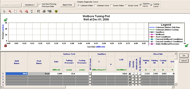
If liquid loading is not considered, proceed to step 2, and note that the pressure drop in the wellbore will be calculated by the single or multiphase correlation in all cases.

If liquid loading should be considered, under the heading Liquid Loading Parameters, select the liquid lift correlation that will be used to predict when the well will load. For more detail on how to choose between the possible correlations, see Sandface C calculations.

The column toggle labeled "Liquid Level Reaches Tubing / Annulus" determines whether a liquid column will form within the tubing / annulus once the well can no longer lift liquids within this segment. For some wells where the perforations are located far below the end of tubing, a liquid column will not reach to the tubing / annulus even after the well can no longer lift liquids.

If it is likely that liquids will accumulate in the tubing, make sure to select the checkbox in the column Liquid Level Reaches Tubing / Annulus . In this case, when the well can no longer lift liquids in the tubing the pressure drop defined by the "∆P in Tub / Ann When Loaded", the column will be applied to the well. However, if the difference between the EOT and MPP is large and it is therefore likely that liquids would accumulate in the casing and never reach the tubing ensure that it says in the column Liquid Level Reaches Tubing / Annulus, then select the Liquid Lift Correlation to use. Scroll to the right and select Multiphase flow, if applicable; then select the appropriate correlation.

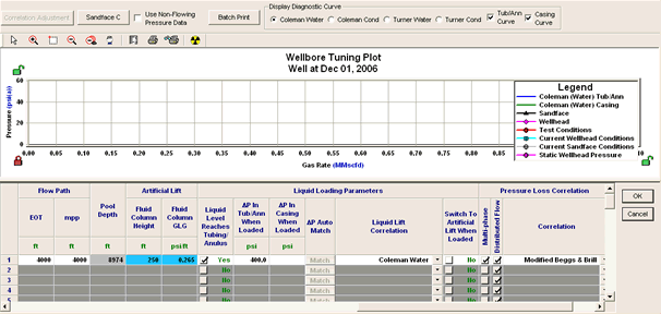
B. Finally, estimate an n-value to account for near wellbore turbulence. For rate wells, an n value close to or equal to 1 should be used. For high flow rate wells, where high velocities in the near wellbore region could be expected to cause additional pressure losses due to turbulence, lower n values, approaching a minimum of 0.5 should be used.

C. Calculate the Sandface C value for the well by clicking the "Sandface C" button (top left corner of the editor).

Scenario 2

The well is not able to lift liquids, and the C-value can be calculated from non-flowing side wellhead conditions

If the flow rate is lower than the flow rate required to lift liquids (this can be determined by the Turner or Coleman liquid lift correlation), liquids will begin to accumulate within the wellbore and create an additional pressure drop that will restrict the well performance, or at times even shut the well in. The Turner or Coleman diagnostic plots, which can be toggled to display in the upper left corner of the Tuning editor, can be used to determine at what rate a well will no longer be able to lift liquids. The curves display the minimum gas rate, as predicted by either the Turner or Coleman liquid lift correlation, whereby liquids would be carried up the wellbore. Using the previous scenario as an example, at the wellhead pressure of 55 psi, we need ~0.25 MMscfd or more of gas flow to lift liquids in the tubing portion of the wellbore. Note that curves for both the tubing / annulus segment and the casing segment of the wellbore are displayed.

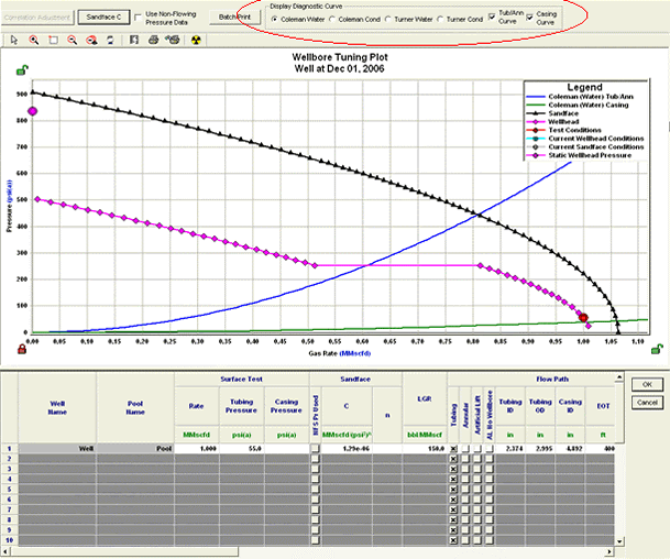
If the flow rate is less then the critical rate, using flowing pressure data to calculate the Sandface deliverability will not be feasible, as the actual flowing pressures will be skewed by the existence of the liquid column in the wellbore.

In such scenarios, if there is no packer downhole, the non-flowing side surface pressure can be used to estimate the bottomhole pressure.

A. Select "Use Non-Flowing Pressure Data" to the right of the Sandface C button.

B. Enter both the current flowing pressure and the non-flowing pressure, as well as the current flow rate.

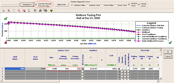
C. Calculate the Sandface C value.

Sandface C will be calculated by extrapolating the non-flowing surface pressure downhole to the end of the tubing. The assumption used is that only a gas gradient exists on the non-flowing side. From the EOT to the MPP, a liquid column exists, and is accounted for with a gradient of 0.265 psi/ft over the length of the casing segment.

Scenario 3

The C-value is known from a prior flow test, but the well is not able to lift liquids, so the C-value is matched to current flowing wellhead conditions by allowing Piper to adjust the effect of liquids in the wellbore.

A. Manually enter a Sandface C

B. Use the Auto Match to match the flowing side pressure and flow rate (shown on the plot with the red circle) to the Sandface C that was entered. The "∆P in Tub / Ann When Loaded" will be adjusted to match the pressure drop between the current surface and sandface condition.

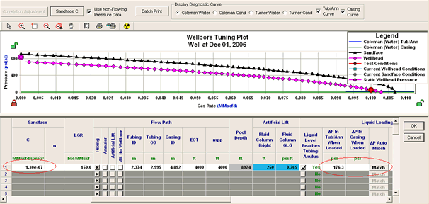
For more information about the calculations, see Sandface C calculations.

For a more detailed description of modeling and options, see Wellbore Tuning Reference Materials.

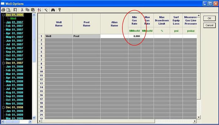
Well options

In the Well Options editor, you can apply flow rate restrictions to wells, impose a maximum drawdown limit, or specify surface equipment losses. If measured line pressures are available, you can enter these values in the Measured Gas Line or Measured Water Line Pressure columns.

Note:

Data entered in the Measured Gas Line Pressure column is not used for calculation purposes, but it is sometimes useful to display this information either on the map or bubble map dialog box. With this information, you can visualize the difference between field reported and model calculated pressures.

Data entered in the Measured Water Line Pressure column is not used for calculation purposes either. This feature is available to monitor the difference between gas line pressures and water line operating pressures on an on-going basis.

If your well shuts in and you cannot get it to produce again, even after reducing the line pressure upstream of the well (to the point where it should produce), try setting the Min Gas Rate to zero in the Well Options editor. Wells that have no production return to production when there are reductions to the line pressure downstream of the well, etc.

Reservoirs editor

With this editor, you can define gas reservoir properties. Although the majority of modeling work typically involves gas reservoirs undergoing volumetric depletion, other drive mechanisms can be modeled such as:

• Pressure support from connected reservoirs
• Pressure support from aquifers
• Over pressured reservoirs

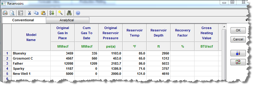
For these more advanced modeling scenarios, data is entered into the Connected Reservoir / Water Drive editor .

For a more detailed description of the reservoir types available, see Reservoirs .

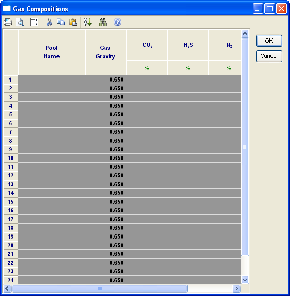
Reservoir Gas Compositions editor

This editor can be accessed either from within the Reservoirs Editor, or on the main toolbar. With this editor, you can enter the reservoir gas composition. When wells are connected to a reservoir, then you have the option to use the reservoir gas composition for that well from the Well Editor. For more information, see Well Fluid Properties.

Connected Reservoir / Water Drive editor

The connected reservoir / water drive model extends the capabilities of the reservoir editor to include non-pressure depleting reservoirs. Reservoir types defined in this editor are:

• Connected reservoirs
• Water drive reservoirs
• Geo-pressured reservoirs

The Connected Reservoir / Water Drive editor is shown below.

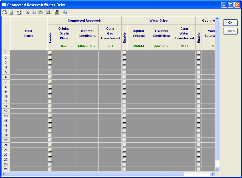
The connected reservoir model (associated tight gas reservoir volumes in intimate contact with the main reservoir gas-in-place) is based on the method developed by David Payne, "Material Balance Calculations in Tight Gas Reservoirs: The Pitfalls of P/Z Plots and a More Accurate Technique", 1996, SPE 36702.

The water drive model is a steady-state solution for water drive reservoirs based on the method put forward by Fetkovich.

The geo-pressure reservoir model accounts for the compressibility effects of connate water and rock.

The connected reservoir / water drive model is designed to model the pressure support of an underlying aquifer using the method derived by Fetkovich. The connected / water drive data inputs work together with inputs from the associated reservoir names in the Reservoirs editor. Guessing for input parameters is not recommended.

For a more detailed description of the reservoir types available, seeReservoirs .

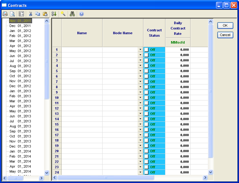
Contracts editor

Contracts are used to restrict flow through a node below a value, which you specify, the contract volume. The contract facility acts as a choke restricting production to a specified volume. Once the field is no longer able to meet the contract requirement, the choke is removed.

Refrigeration Plants editor

Refrigeration plants are used to remove natural gas liquids (NGLs) from the gas stream entering a node. The amount of liquids removed can be specified in one of two ways:

1. Liquid Yields - you specify the liquid yield (bbls/mmcfd) for a specific NGL component. This option is available when a simplified gas analysis is used.

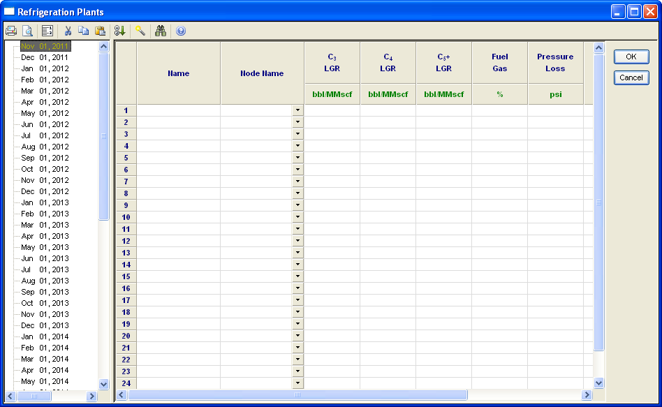
2. Recovery Efficiency - you can specify the fraction of each component that is removed from the raw gas stream. This option is available when a detailed gas analysis is used.

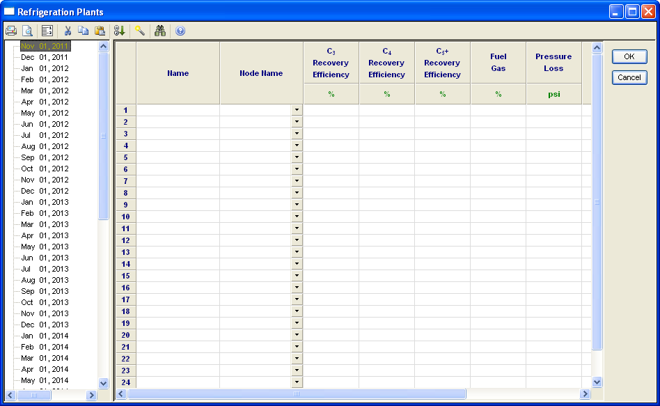
With the refrigeration editor, you can also specify fuel gas requirements expressed as a percentage of throughput volume, and pressure losses across the facility, if applicable.

For a more detailed description of refrigeration modeling and options, see Refrigeration .

Amines editor

Amine plants are used to remove acid gas components from a raw gas stream. In this editor, you can specify the percentage of acid gas components to remove, fuel gas, and pressure losses through the facility.

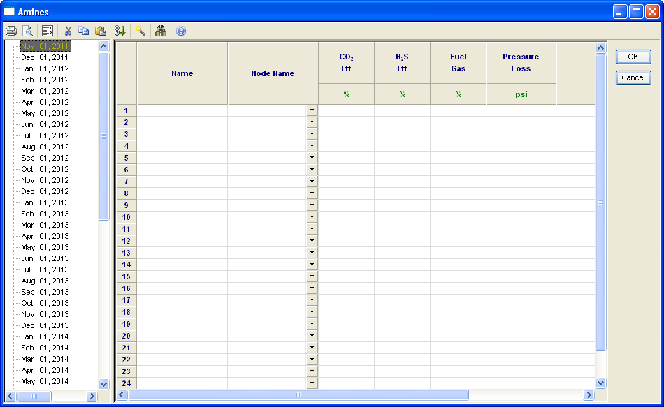
For a more detailed description of amine modeling and options, see Amine separators.

Intakes / Offtakes editor

With Piper, you can incorporate gas volume additions from facilities other than wells (intakes), and withdrawals to multiple delivery and/or sales points (offtakes).

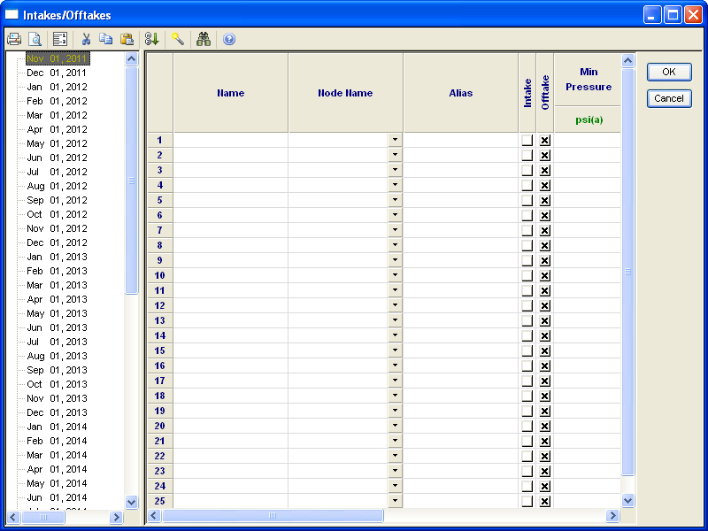
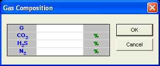
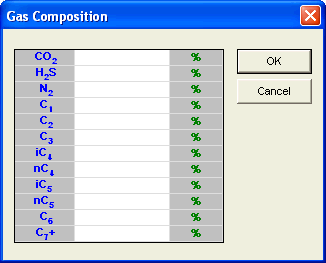
With intake facilities, you can enter a fixed volume of gas into a system. You can define the composition of the injected gas in the Gas Props column: either a simple or detailed analysis can be selected.

Simple analysis

Detailed analysis

To enable this analysis, click the Forecast Options menu, and select Composition Tracking.

Offtakes provide you with the flexibility to incorporate several delivery points into a single model. An offtake requires a fixed gas rate and a minimum delivery pressure to be specified. If the specified rate cannot be maintained, at or above the minimum delivery pressure, the offtake facility is automatically disabled. If the staging option is selected, the offtake facility continues to accept gas, at a reduced rate, while maintaining the specified minimum delivery pressure.

For a more detailed description of modeling and options, see Intakes and Offtakes.

Pressure Loss editor

With Piper, you can assign additional pressure losses to any point in a gathering system.

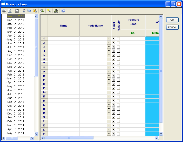
Once a location has been defined, you can choose either a fixed or variable pressure loss. Fixed pressure losses stay constant through time and require the pressure loss to be specified. Variable pressure losses change in accordance with production rates, and you are required to enter the pressure loss, gas rate, and outlet pressure. These parameters are entered for the initial month the variable pressure loss is introduced.

For a more detailed description of modeling and options, see Pressure Losses.

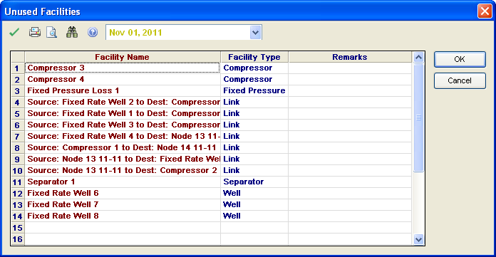
Unused Facilities

Unused facilities are displayed in this dialog box. If there are a lot of entries in this dialog box, it is a good idea to check the system links. When equipment is disconnected, other linked items can also become disconnected.

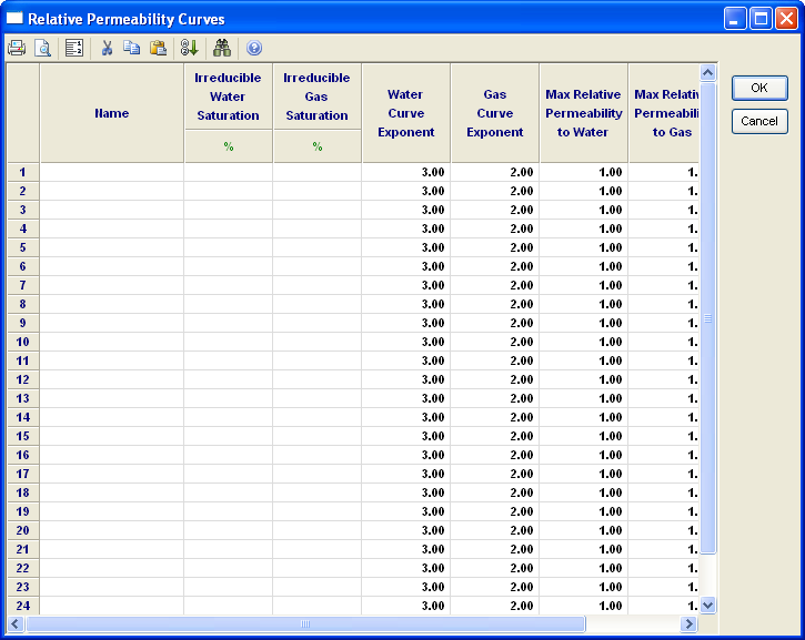
Relative Permeability Curves editor

To open the Relative Permeability editor, click its icon. This editor is automatically populated with parameters from importing history-matched wells from Harmony Enterprise. Percent irreducible water and gas saturation, water and gas curve exponent, and maximum relative permeability to water and gas are specified in this editor.

Default dialog box editor

The Default dialog box editor sets the default values for many of the properties and units used by Piper.

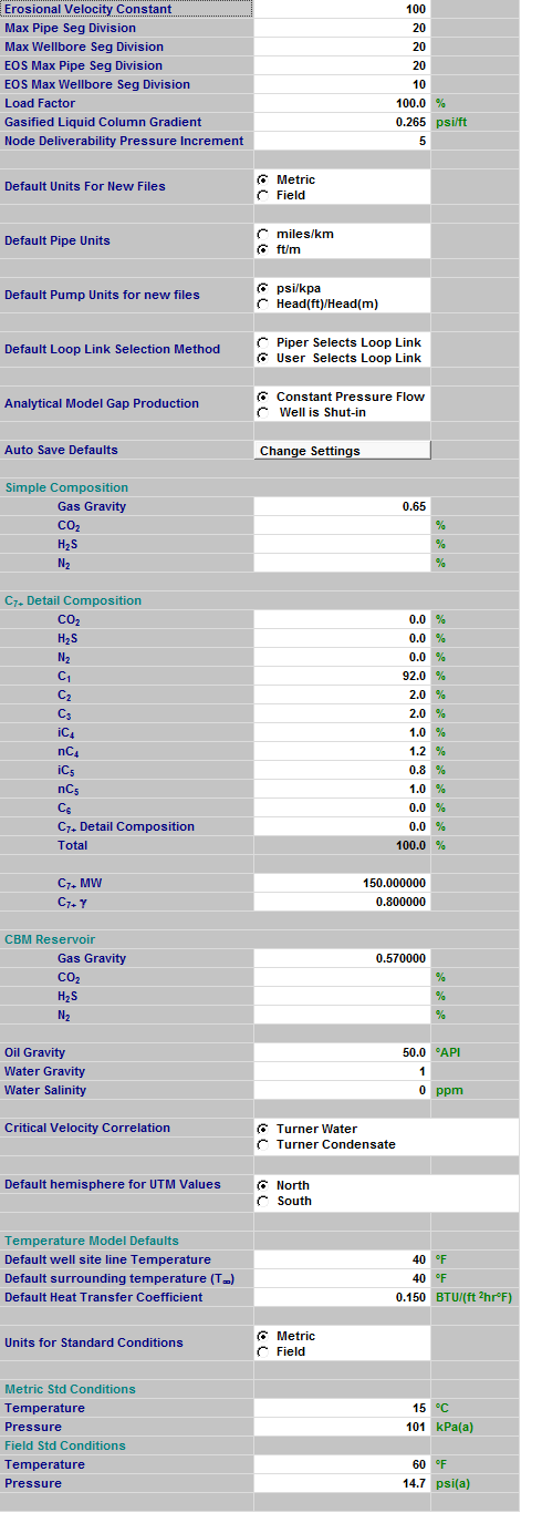
For information on these fields, see defaults.